Function Graph
Overview
The Function Graph dynamically plots function curves based on user-input mathematical expressions. It's a specialized widget for visualizing functions directly within a Panel Card. This interactive visualization is especially useful for illustrating theoretical function behavior and exploring parameter sensitivities directly within your experiment dashboards.
Key Features
- Dynamic Formula Parameters: Use runtime values from other Form controls (e.g., Sliders, Number Inputs) on the same dashboard as dynamic parameters directly within your function expressions.
- Real-Time Plotting: As you adjust these controls, the function graph updates instantly, allowing you to see how parameter changes affect the curve's shape.
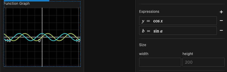
- Multiple Expressions: Display several function curves overlaid on the same graph by adding multiple expressions.
- Customizable Coordinate System:
- Set custom ranges for the X and Y axes.
- Supports both linear and logarithmic scales for the axes.
- Graph Navigation:
- Zoom: Use the mouse scroll wheel, or hold
Shift+Left Mouse Buttonand drag. - Pan: Hold
Spacebar+Left Mouse Buttonand drag.
- Zoom: Use the mouse scroll wheel, or hold
It's important to understand the distinction:
- Function Graph
- Input: Directly plots mathematical expressions (formulas).
- Rendering: Generates and displays curves immediately based on these formulas.
- Use Case: Ideal for visualizing theoretical function shapes, exploring mathematical relationships, or observing parameter sensitivity in real-time without running a full simulation.
- Chart Cards
- Input: Visualizes data generated from a simulation run (i.e., data that already exists in a
Datatable). - Rendering: Displays this pre-existing data.
- Use Case: Best for presenting the results of model simulations, showing how outputs change over time or according to different states.
- Input: Visualizes data generated from a simulation run (i.e., data that already exists in a
Configuration Steps
Beyond the general widget settings (like Label and initial State), the following steps outline the specific configurations for the Function Graph.
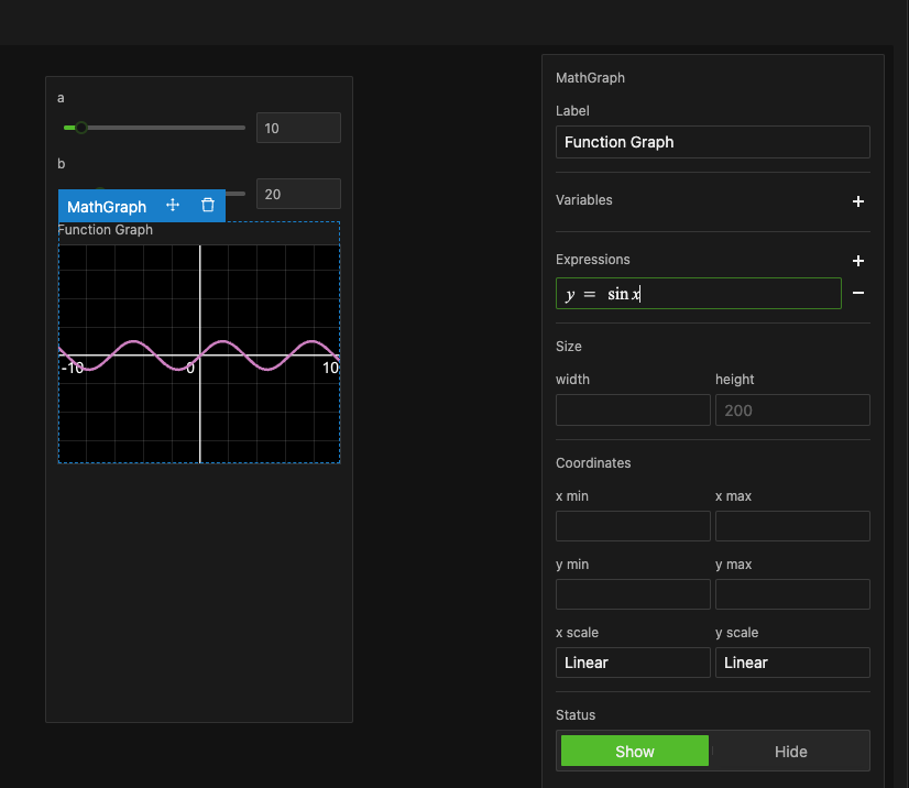
Defining Expressions
- Add or Remove Expressions
- Click the "+" button to add a new expression input field. Multiple expressions can be added—each renders as an independent curve.
- Click the "-" button next to an expression to remove it.
- Input Expressions
- Type the mathematical expression defining the Y-axis value in terms of the X-axis (e.g.,
y = x^2,y = sin(x)). - The graph updates in real time as you type.
- Type the mathematical expression defining the Y-axis value in terms of the X-axis (e.g.,
The widget is powered by the Desmos graphing engine. For detailed syntax and advanced mathematical expression support, refer to the official Desmos documentation.
Binding Variables to Form Controls
You can make your function graphs dynamic by linking variables within your expressions to other Form controls (like Sliders or Number Inputs) within the same Dashboard.
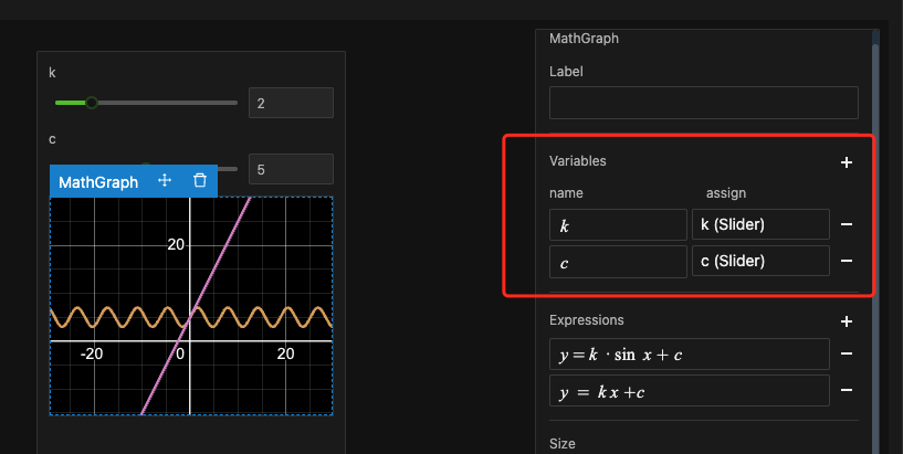
- Add a Variable: Click the "+" to add a new variable entry. (Click "-" to remove one).
- Name the Variable: In the "name" field, enter a name for your variable (e.g.,
k,c). This name will be used in your expressions. - Assign a Control
- From the "assign" dropdown list, select the widget (Global Panel or other widgets which must have a
Labelset, excluding Buttons) that will provide the value for this variable. - Example: If you have a Slider labeled "k", you would select
k (Slider)here.
- From the "assign" dropdown list, select the widget (Global Panel or other widgets which must have a
- Dynamic Updates
- Once bound, whenever you adjust the linked Form Control widget (e.g., move the
k (Slider)), the Graph will automatically re-render, reflecting the new variable value in the plotted curve(s).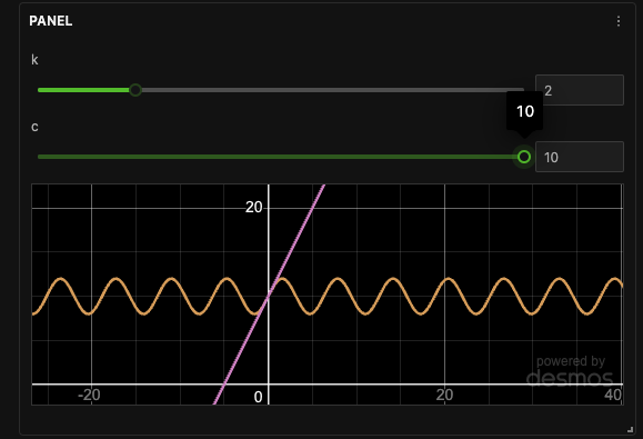
- Once bound, whenever you adjust the linked Form Control widget (e.g., move the
After binding, you can directly use the variable names (e.g., k, c) in your expression input fields (e.g., y = k * sin(x) + c). These variables will act as parameters in your function, dynamically controlled by the linked widgets.
Setting Graph Size
You can specify the width and height of the graph area.
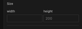
| Setting | Default Value | Description |
|---|---|---|
width | Auto-fits to panel or layout container | Automatically adjusts to container width. You can also manually specify width in pixels if required. |
height | 200 px | Sets the height in pixels. Can be any integer. |
Configuring the Coordinate System
Define the visible range and scale type for the X and Y axes.
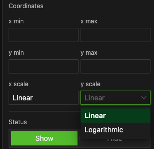
- Set Axis Ranges
- Define the minimum and maximum values for the horizontal axis (Xmin / Xmax) and the vertical axis (Ymin / Ymax).
- Choose Scale Type
- For each axis (
x scale,y scale), you can switch between:- Linear (Default)
- Logarithmic
- For each axis (
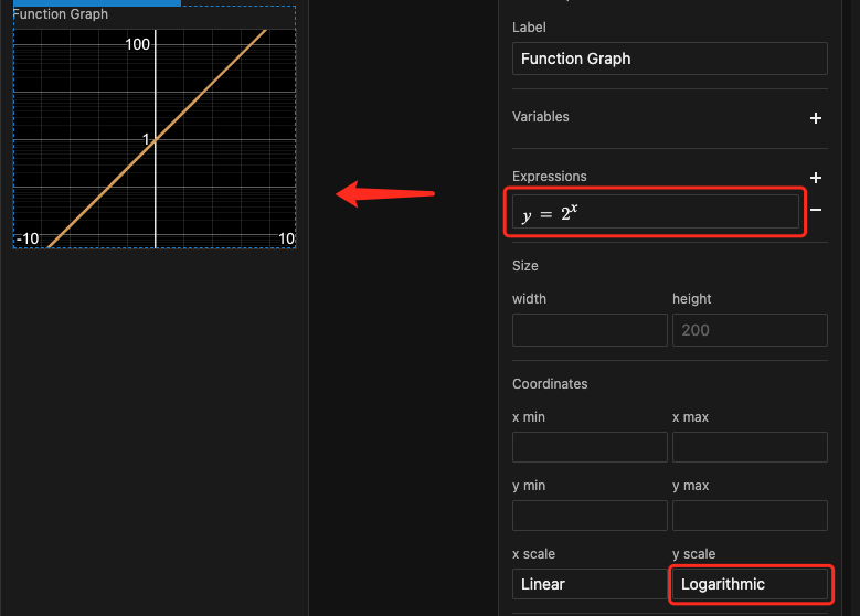
A logarithmic scale is particularly useful for observing exponential or power-law functions, as they will appear as straight lines, making it easier to compare relative growth or changes.
As shown above, switching the Y-axis to a logarithmic scale for an exponential function y = 2ˣ linearises the plot. Likewise, in DeFi scenarios, e.g., visualizing a bonding curve, parameter values bound to UI variables reveal their influence on the curve's shape.
For hands-on bonding-curve examples, see the Parameter Exploration chapter.
Example
In the experiment linked below, you can select different function types and adjust their parameters using Form controls. Observe how the Function Graph updates in real-time: